WASP-69 with HPF: joint stellar/telluric tuning#
WASP-69 makes a great demo because it has a very low \(v\sin{i}\) of 2.2 km/s, which means that its spectral lines appear exceptionally sharp. Here we will analyze a single (noisy) spectrum of WASP-69 observed with HPF.
[1]:
%config Completer.use_jedi = False
[2]:
import torch
from blase.emulator import SparseLogEmulator, ExtrinsicModel, InstrumentalModel
import matplotlib.pyplot as plt
from gollum.phoenix import PHOENIXSpectrum
from gollum.telluric import TelFitSpectrum
from blase.utils import doppler_grid
import astropy.units as u
import numpy as np

if torch.cuda.is_available():
    device = "cuda"
else:
    device = "cpu"

%matplotlib inline
%config InlineBackend.figure_format='retina'
[3]:
device
[3]:
'cuda'
Pre-process the data#
We will quickly pre-process the HPF spectrum with the muler library
[4]:
from muler.hpf import HPFSpectrum
[5]:
raw_data = HPFSpectrum(file='../../data/HPF/WASP-69/Goldilocks_20191019T015252_v1.0_0002.spectra.fits', order=2)
[6]:
data = raw_data.sky_subtract().trim_edges().remove_nans().deblaze().normalize(normalize_by='peak')
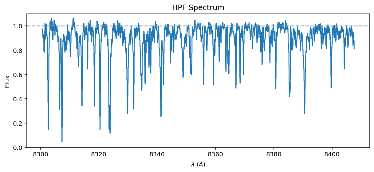
[7]:
ax = data.plot(yhi=1.1);
ax.axhline(1.0, color='#95a5a6', linestyle='dashed');
[8]:
wl_lo = 8300-30.0
wl_hi = 8420+30.0
wavelength_grid = doppler_grid(wl_lo, wl_hi)
Retrieve the Phoenix model#
WASP-69 has \(T_{\mathrm{eff}}=4700\;K\) and \(\log{g}=4.5\), according to sources obtained through NASA Exoplanet Archive (Bonomo et al. 2017, Stassun et al. 2017, Anderson et al. 2014, and references therein). Let’s start with a PHOENIX model possessing these properties.
[9]:
spectrum = PHOENIXSpectrum(teff=4700, logg=4.5, wl_lo=wl_lo, wl_hi=wl_hi)
spectrum = spectrum.divide_by_blackbody()
spectrum = spectrum.normalize()
continuum_fit = spectrum.fit_continuum(polyorder=5)
spectrum = spectrum.divide(continuum_fit, handle_meta="ff")
Retrieve the TelFit Telluric model#
Let’s pick a precomputed TelFit model with comparable temperature and humidity as the data. You can improve on your initial guess by tuning a TelFit model from scratch. We choose to skip this laborious step here, but encourage practitioners to try it on their own.
[10]:
data.meta['header']['ENVTEM'], data.meta['header']['ENVHUM'] # Fahrenheit and Relative Humidity
[10]:
(64.38, 39.601)
That’s about 290 Kelvin and 40% humidity.
[11]:
web_link = 'https://utexas.box.com/shared/static/3d43yqog5htr93qbfql3acg4v4wzhbn8.txt'
[12]:
telluric_spectrum_full = TelFitSpectrum(path=web_link).air_to_vacuum()
mask = ((telluric_spectrum_full.wavelength.value > wl_lo) &
        (telluric_spectrum_full.wavelength.value < wl_hi) )
telluric_spectrum = telluric_spectrum_full.apply_boolean_mask(mask)
telluric_wl = telluric_spectrum.wavelength.value
telluric_flux = np.abs(telluric_spectrum.flux.value)
telluric_lnflux = np.log(telluric_flux) # "natural log" or log base `e`
telluric_lnflux[telluric_lnflux < -15] = -15
Initial guess#
[13]:
system_RV = -9.5 #km/s
BERV = data.estimate_barycorr().to(u.km/u.s).value
observed_RV = system_RV - BERV#km/s
vsini = 2.2 #km/s
resolving_power = 55_000
initial_guess = spectrum.resample_to_uniform_in_velocity()\
                        .rv_shift(observed_RV)\
                        .rotationally_broaden(vsini)\
                        .instrumental_broaden(resolving_power)\
                        .resample(data)

initial_telluric = telluric_spectrum.instrumental_broaden(resolving_power)\
                                         .resample(data)
[14]:
ax = data.plot(label='data')
initial_telluric.plot(ax=ax, label='TelFit (Initial)')
initial_guess.plot(ax=ax, label='WASP-69 (Initial)')
ax.legend(ncol=3);
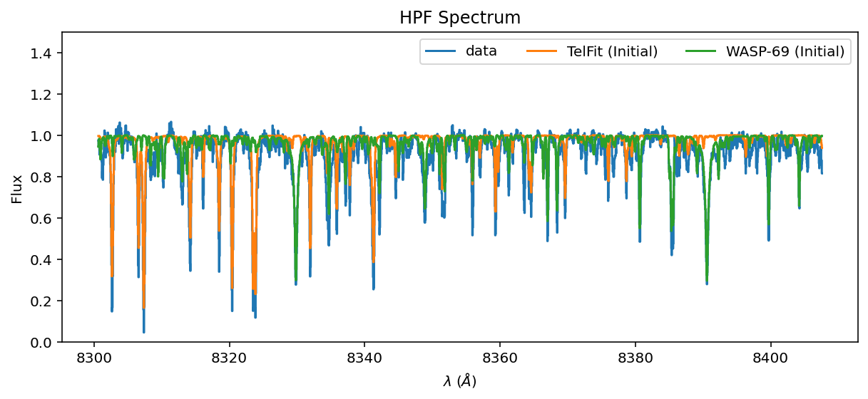
Ok, the lines are in the right place, but the amplitudes are inexact. Let’s tune them with blase!
Clone the stellar and telluric model#
[15]:
stellar_emulator = SparseLogEmulator(spectrum.wavelength.value,
                                     np.log(spectrum.flux.value), prominence=0.01, device=device)
stellar_emulator.to(device)
/home/gully/GitHub/blase/src/blase/emulator.py:360: UserWarning: To copy construct from a tensor, it is recommended to use sourceTensor.clone().detach() or sourceTensor.clone().detach().requires_grad_(True), rather than torch.tensor(sourceTensor).
  self.target = torch.tensor(
Initializing a sparse model with 290 spectral lines
[15]:
SparseLogEmulator()
[16]:
telluric_emulator = SparseLogEmulator(telluric_spectrum.wavelength.value,
                                      np.log(telluric_spectrum.flux.value),
                                      prominence=0.01, device=device)
telluric_emulator.to(device)
Initializing a sparse model with 148 spectral lines
[16]:
SparseLogEmulator()
Fine-tune the clone#
[17]:
stellar_emulator.optimize(epochs=1000, LR=0.01)
Training Loss: 0.00010681: 100%|██████████████████████████| 1000/1000 [00:04<00:00, 212.86it/s]
[18]:
telluric_emulator.optimize(epochs=1000, LR=0.01)
Training Loss: 0.00000873: 100%|██████████████████████████| 1000/1000 [00:04<00:00, 231.39it/s]
Step 3: Extrinsic model#
[19]:
extrinsic_layer = ExtrinsicModel(wavelength_grid, device=device)
vsini = torch.tensor(vsini)
extrinsic_layer.ln_vsini.data = torch.log(vsini)
extrinsic_layer.to(device)
[19]:
ExtrinsicModel()
(Remap the stellar and telluric emulator to a standardized wavelength grid).
[20]:
stellar_emulator = SparseLogEmulator(wavelength_grid,
                                     init_state_dict=stellar_emulator.state_dict(), device=device)
stellar_emulator.radial_velocity.data = torch.tensor(observed_RV)
stellar_emulator.to(device)
telluric_emulator = SparseLogEmulator(wavelength_grid,
                                     init_state_dict=telluric_emulator.state_dict(), device=device)
telluric_emulator.to(device)
Initializing a sparse model with 290 spectral lines
Initializing a sparse model with 148 spectral lines
[20]:
SparseLogEmulator()
Forward model#
[21]:
stellar_flux = stellar_emulator.forward()
broadened_flux = extrinsic_layer(stellar_flux)
telluric_attenuation = telluric_emulator.forward()
Joint telluric and stellar model#
[22]:
flux_at_telescope = broadened_flux * telluric_attenuation
Instrumental model#
[23]:
instrumental_model = InstrumentalModel(data.bin_edges.value, wavelength_grid, device=device)
instrumental_model.to(device)
[23]:
InstrumentalModel(
  (linear_model): Linear(in_features=15, out_features=1, bias=True)
)
[24]:
instrumental_model.ln_sigma_angs.data = torch.log(torch.tensor(0.064))
[25]:
detector_flux = instrumental_model.forward(flux_at_telescope)
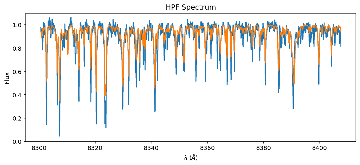
[26]:
ax = data.plot(yhi=1.1)
ax.step(data.wavelength, detector_flux.detach().cpu().numpy());
#ax.set_xlim(8320, 8340)
Transfer learn a semi-empirical model#
Here we compare the resampled joint model to the observed data to “transfer learn” underlying super resolution spectra.
[27]:
from torch import nn
from tqdm import trange
import torch.optim as optim
[28]:
data_target = torch.tensor(
    data.flux.value.astype(np.float64), device=device, dtype=torch.float64
)

data_wavelength = torch.tensor(
    data.wavelength.value.astype(np.float64), device=device, dtype=torch.float64
)
[29]:
loss_fn = nn.MSELoss(reduction="mean")
Fix certain parameters, allow others to vary#
As we have seen before, you can fix parameters by “turning off their gradients”. We will start by turning off ALL gradients. Then turn on some.
[47]:
stellar_emulator.amplitudes.requires_grad = True
stellar_emulator.radial_velocity.requires_grad = True
telluric_emulator.amplitudes.requires_grad = True
instrumental_model.ln_sigma_angs.requires_grad = True
[48]:
optimizer = optim.Adam(
    list(filter(lambda p: p.requires_grad, stellar_emulator.parameters()))
    + list(filter(lambda p: p.requires_grad, telluric_emulator.parameters()))
    + list(filter(lambda p: p.requires_grad, extrinsic_layer.parameters()))
    + list(filter(lambda p: p.requires_grad, instrumental_model.parameters())),
    0.01,
    amsgrad=True,
)
[54]:
n_epochs = 2000
losses = []
Regularization is fundamental#
The blase model as it stands is too flexible. It must have regularization to balance its propensity to overfit.
First, we need to assign uncertainty to the data in order to weigh the prior against new data:
[55]:
# We need uncertainty to be able to compute the posterior
# Assert fixed per-pixel uncertainty for now
per_pixel_uncertainty = torch.tensor(0.01, device=device, dtype=torch.float64)
Then we need the prior. For now, let’s just apply priors on the amplitudes (almost everything else is fixed). We need to set the regularization hyperparameter tuning.
[56]:
stellar_amp_regularization = 5.1
telluric_amp_regularization = 5.1
[57]:
import copy
[58]:
with torch.no_grad():
    stellar_init_amps = copy.deepcopy(stellar_emulator.amplitudes)
    telluric_init_amps = copy.deepcopy(telluric_emulator.amplitudes)

# Define the prior on the amplitude
def ln_prior(stellar_amps, telluric_amps,):
    """
    Prior for the amplitude vector
    """
    amp_diff1 = stellar_init_amps - stellar_amps
    ln_prior1 = 0.5 * torch.sum((amp_diff1 ** 2) / (stellar_amp_regularization ** 2))

    amp_diff2 = telluric_init_amps - telluric_amps
    ln_prior2 = 0.5 * torch.sum((amp_diff2 ** 2) / (telluric_amp_regularization ** 2))

    return ln_prior1 + ln_prior2
[59]:
t_iter = trange(n_epochs, desc="Training", leave=True)
for epoch in t_iter:
    stellar_emulator.train()
    telluric_emulator.train()
    extrinsic_layer.train()
    instrumental_model.train()

    stellar_flux = stellar_emulator.forward()
    broadened_flux = extrinsic_layer(stellar_flux)
    telluric_attenuation = telluric_emulator.forward()
    flux_at_telescope = broadened_flux * telluric_attenuation
    detector_flux = instrumental_model.forward(flux_at_telescope)

    loss = loss_fn(detector_flux / per_pixel_uncertainty, data_target / per_pixel_uncertainty)
    loss += ln_prior(stellar_emulator.amplitudes, telluric_emulator.amplitudes)
    loss.backward()
    optimizer.step()
    optimizer.zero_grad()
    t_iter.set_description("Training Loss: {:0.8f}".format(loss.item()))
Training Loss: 8.60397831: 100%|███████████████████████████| 2000/2000 [02:43<00:00, 12.24it/s]
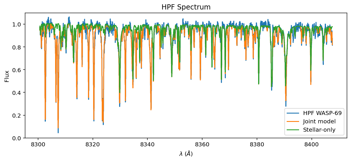
Spot check the transfer-learned joint model#
[60]:
ax = data.plot(yhi=1.1, label='HPF WASP-69')
ax.step(data.wavelength, detector_flux.detach().cpu().numpy(), label='Joint model');
ax.step(data.wavelength, instrumental_model.forward(broadened_flux).detach().cpu().numpy(),
       label='Stellar-only');
ax.legend()
[60]:
<matplotlib.legend.Legend at 0x7f5a26264a00>
[61]:
ax = data.plot(yhi=1.1)
ax.step(data.wavelength, detector_flux.detach().cpu().numpy());
ax.set_xlim(8320, 8340)
[61]:
(8320.0, 8340.0)
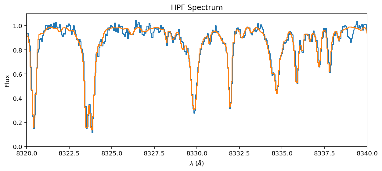
Don’t get too excited! This performance is very overfit. It needs regularization!
Inspect the individual stellar and telluric components#
[62]:
with torch.no_grad():
    stellar_emulator.radial_velocity.data *=0
    stellar_post = stellar_emulator.forward().cpu().numpy()
    telluric_post = telluric_emulator.forward().cpu().numpy()
[63]:
ax = spectrum.plot(ylo=0, yhi=1.1, label='Native PHOENIX')
ax.step(wavelength_grid, stellar_post, label='Transfer learned');
ax.legend()
ax.set_xlim(8320, 8340);
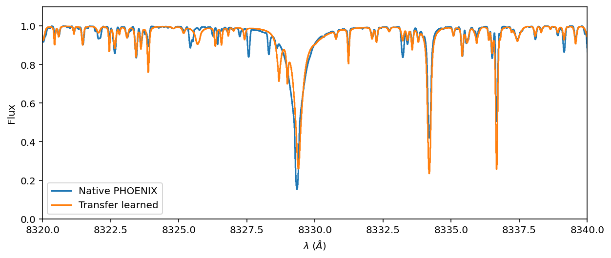
You can see that the telluric and stellar models compensated for imperfections in the line wings by overbloating the amplitudes of bystander lines. This unlikely tradeoff makes sense once the line is convolved with an instrument kernel.
[64]:
ax = telluric_spectrum.plot(ylo=0, yhi=1.1, label='Native TelFit')
ax.step(wavelength_grid, telluric_post, label='Transfer learned');
ax.legend()
ax.set_xlim(8320, 8340);
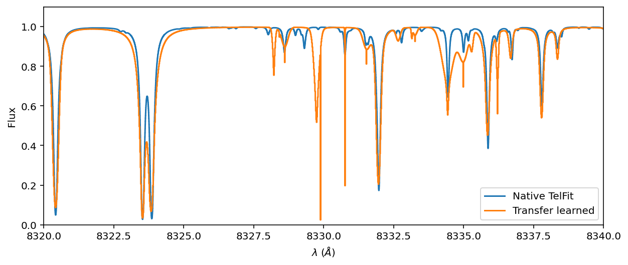
Voilá! We did it! We tuned the telluric and stellar line amplitudes simultaneously with real high resolution data. We notice a few remaining inperfections. Here are the next steps to fix those imperfections:
- Overall fit quality and hyperparameter tuningFirst, the fit quality isn’t great. We probably want to tune the regularization to learn from the data a bit more than the model. This tuning is the trickiest hyperparameter to get right in blasé.
- Expand regularization to include all other parametersWe are only tuning amplitudes right now (and RV and instrumental resolution). Let’s tune and regularize all of the parameters (in a judicious way).
- More flexible super-Lorentzian shapesThe broad and deep stellar lines depart significantly from their expectations in the PHOENIX models. In those cases, we want to allow the line widths to adapt. But even if we allowed the linewings to float, the updates will likely fall short of reality. We should make the line widths more flexible, as described in the paper.
- Start with a better templateIdeally you want to start with the best possible template, the precomputed synthetic spectral model that most closely resembles your spectrum a-priori. We should especially strive for this goal with TelFit, which offers fine-tuning. In particular, we should adapt the Earth’s \(P-T\) profile to match reality, instead of the static template we default to. We may also be slightly wrong in terms of the number of layers of the atmosphere, and how it rounds the dense final layer closest to the Observatory.
- Train for longerSimply training for longer than mitigate some poor initialization artifacts. You have to be a bit careful, since early-stopping can act as a form of regularization too.