Step 3: Stellar rotational broadening and RV shifting

The emergent spectrum of a star gets modulated by at least two extrinsic parameters—\(v\sin{i}\) and \(RV\)—before entering our metaphorical orbit. Here we show how to modulate a cloned stellar model with these two parameters.

import torch
from blase.emulator import SparseLinearEmulator, SparseLogEmulator, ExtrinsicModel
from blase.utils import doppler_grid
import matplotlib.pyplot as plt
import math
%config InlineBackend.figure_format='retina'

wl_lo = 11_000-60
wl_hi = 11_180+60
wavelength_grid = doppler_grid(wl_lo, wl_hi)

if torch.cuda.is_available():
    device = "cuda"
else:
    device = "cpu"

We will fetch the pretrained stellar model, following the previous tutorial.

stellar_pretrained_model = torch.load('phoenix_clone_T4700g4p5_prom0p01_11000Ang.pt')

stellar_emulator = SparseLinearEmulator(wavelength_grid,
                                        init_state_dict=stellar_pretrained_model)

Initializing a sparse model with 426 spectral lines

y0 = stellar_emulator.forward().detach().cpu().numpy()

Set the \(v\sin{i}\) and \(RV\) for the extrinsic model

extrinsic_layer = ExtrinsicModel(wavelength_grid, device=device)

We set natural log of the rotational broadening for numerical purposes.

vsini = torch.tensor(11.1)
extrinsic_layer.ln_vsini.data = torch.log(vsini)

For technical and historical reasons, the radial velocity augments the stellar emulator.

Ideally this change would live instead under the ExtrinsicModel umbrella, and we are contemplating making that change.

RV = torch.tensor(-5.6789)
stellar_emulator.radial_velocity.data = RV

Key idea: The output of one model is the input to the next

The symmetry should feel wholesome: the stellar forward model goes into the extrinsic model, as if it were an anonymous component on a factory conveyorbelt.

stellar_flux = stellar_emulator.forward()
modulated_flux = extrinsic_layer(stellar_flux)

Recall that both layers have tunable parameters, and PyTorch stores the order of operations in its memory.

(For plotting purposes we have to “detach” from this over-zealous memory, and ensure that the data is on a cpu.)

y1 = stellar_flux.detach().cpu().numpy()
y2 = modulated_flux.detach().cpu().numpy()

plt.figure(figsize=(8, 5))
plt.step(wavelength_grid, y0, label='Unperturbed stellar clone')
plt.step(wavelength_grid, y1, label=f'RV-shifted by {RV:0.2f} km/s')
plt.xlim(11_098.2, 11_099.7); plt.ylim(0.7, 1.05)
plt.legend();

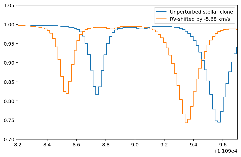
Neat! Notice how the pixel coordinates stay in the same place, but the line-center positions change the fluxes evaluated at those coordinates. The spectrum is not merely a translation of coordinates, its a re-evaluation of the coordinates with new line center positions. This design choice ensures that the radial velocity is “auto-differentiable”.

plt.figure(figsize=(8, 5))
plt.step(wavelength_grid, y1, label=f'RV-shifted by {RV:0.2f} km/s')
plt.step(wavelength_grid, y2, label=f'Rotationally Broadened ')
plt.xlim(11_070, 11_100)
plt.legend();

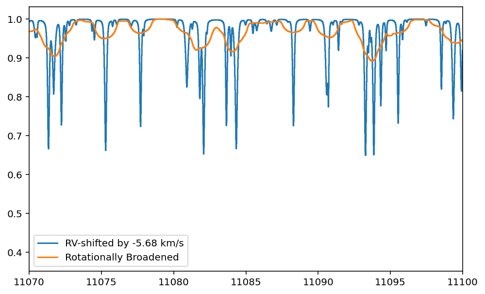
Voilá! We successfully modulated the cloned spectrum with both rotational broadening and radial_velocity. We have not yet shown the full power of this technique: through the “magic” of autodiff, these physically interpretable values can get updated simultaneously as the line strengths themselves are all perturbed. We will see this tuning in the next step.