WASP-69 with HPF Paper Figures:#

Joint stellar/telluric tuning#

August 4, 2022: Work in progress!

This notebook is merely a copy of our Deep Dive on WASP-69, with the figures updated and annotated for publication quality. Enjoy!

[1]:

%config Completer.use_jedi = False

[2]:

import torch
from blase.emulator import SparseLogEmulator, ExtrinsicModel, InstrumentalModel
import matplotlib.pyplot as plt
from gollum.phoenix import PHOENIXSpectrum
from gollum.telluric import TelFitSpectrum
from blase.utils import doppler_grid
import astropy.units as u
import numpy as np

if torch.cuda.is_available():
    device = "cuda"
else:
    device = "cpu"

%matplotlib inline
%config InlineBackend.figure_format='retina'

[3]:

device

[3]:

'cuda'

Pre-process the data#

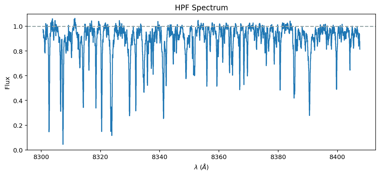
We will quickly pre-process the HPF spectrum with the muler library

[4]:

from muler.hpf import HPFSpectrum

[5]:

raw_data = HPFSpectrum(file='../../data/HPF/WASP-69/Goldilocks_20191019T015252_v1.0_0002.spectra.fits', order=2)

[6]:

data = raw_data.sky_subtract().trim_edges().remove_nans().deblaze().normalize(normalize_by='peak')

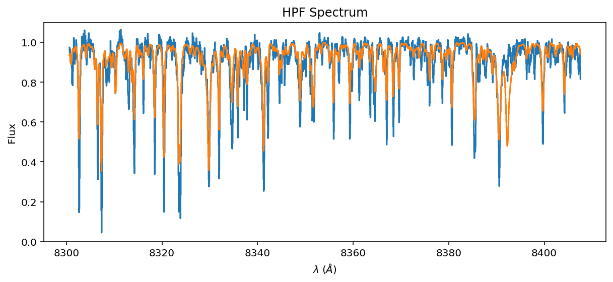
[7]:

ax = data.plot(yhi=1.1);
ax.axhline(1.0, color='#95a5a6', linestyle='dashed');

../_images/paper_figures_WASP-69_HPF_paperfigs_10_0.png

[8]:

wl_lo = 8300-30.0
wl_hi = 8420+30.0
wavelength_grid = doppler_grid(wl_lo, wl_hi)

Retrieve the Phoenix model#

WASP-69 has \(T_{\mathrm{eff}}=4700\;K\) and \(\log{g}=4.5\), according to sources obtained through NASA Exoplanet Archive (Bonomo et al. 2017, Stassun et al. 2017, Anderson et al. 2014, and references therein). Let’s start with a PHOENIX model possessing these properties.

[9]:

spectrum = PHOENIXSpectrum(teff=4700, logg=4.5, wl_lo=wl_lo, wl_hi=wl_hi)
spectrum = spectrum.divide_by_blackbody()
spectrum = spectrum.normalize()
continuum_fit = spectrum.fit_continuum(polyorder=5)
spectrum = spectrum.divide(continuum_fit, handle_meta="ff")

Retrieve the TelFit Telluric model#

Let’s pick a precomputed TelFit model with comparable temperature and humidity as the data. You can improve on your initial guess by tuning a TelFit model from scratch. We choose to skip this laborious step here, but encourage practitioners to try it on their own.

[10]:

data.meta['header']['ENVTEM'], data.meta['header']['ENVHUM'] # Fahrenheit and Relative Humidity

[10]:

(64.38, 39.601)

That’s about 290 Kelvin and 40% humidity.

[11]:

web_link = 'https://utexas.box.com/shared/static/3d43yqog5htr93qbfql3acg4v4wzhbn8.txt'

[12]:

telluric_spectrum_full = TelFitSpectrum(path=web_link).air_to_vacuum()
mask = ((telluric_spectrum_full.wavelength.value > wl_lo) &
        (telluric_spectrum_full.wavelength.value < wl_hi) )
telluric_spectrum = telluric_spectrum_full.apply_boolean_mask(mask)
telluric_wl = telluric_spectrum.wavelength.value
telluric_flux = np.abs(telluric_spectrum.flux.value)
telluric_lnflux = np.log(telluric_flux) # "natural log" or log base `e`
telluric_lnflux[telluric_lnflux < -15] = -15

Initial guess#

[13]:

system_RV = -9.5 #km/s
BERV = data.estimate_barycorr().to(u.km/u.s).value
observed_RV = system_RV - BERV#km/s
vsini = 2.2 #km/s
resolving_power = 55_000
initial_guess = spectrum.resample_to_uniform_in_velocity()\
                        .rv_shift(observed_RV)\
                        .rotationally_broaden(vsini)\
                        .instrumental_broaden(resolving_power)\
                        .resample(data)

initial_telluric = telluric_spectrum.instrumental_broaden(resolving_power)\
                                         .resample(data)

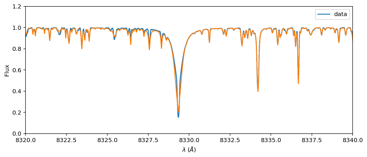
[14]:

ax = data.plot(label='data')
initial_telluric.plot(ax=ax, label='TelFit (Initial)')
initial_guess.plot(ax=ax, label='WASP-69 (Initial)')
ax.legend(ncol=3);

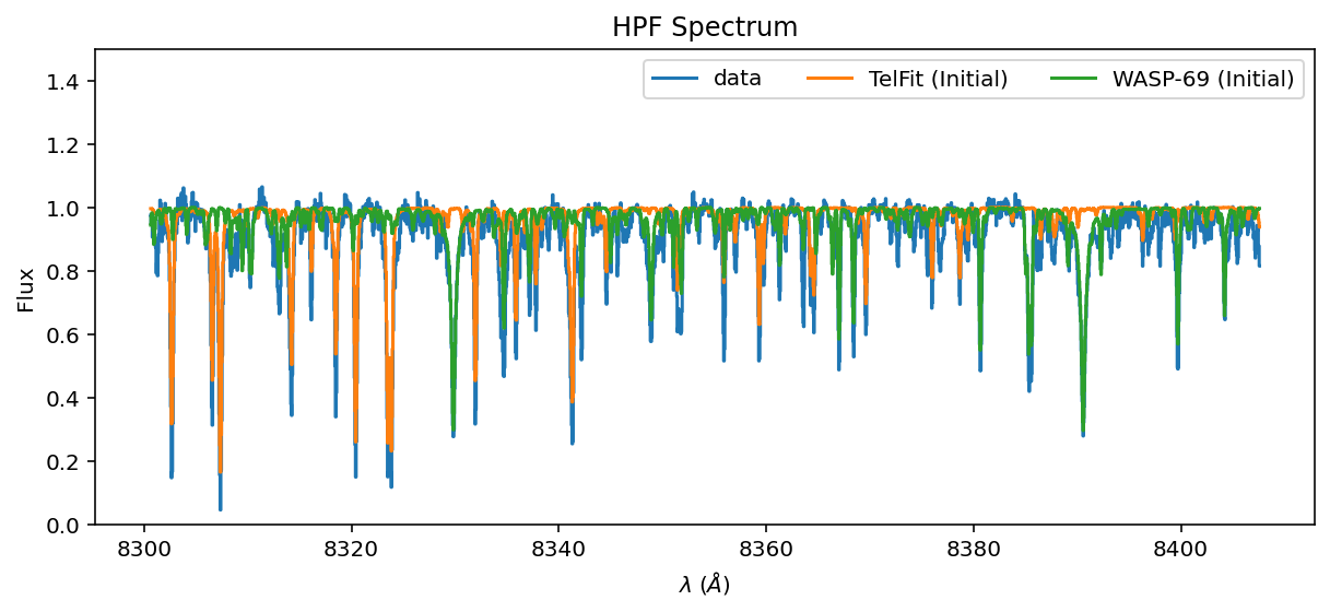
../_images/paper_figures_WASP-69_HPF_paperfigs_21_0.png

Ok, the lines are in the right place, but the amplitudes are inexact. Let’s tune them with blase!

Clone the stellar and telluric model#

[15]:

stellar_emulator = SparseLogEmulator(spectrum.wavelength.value,
                                     np.log(spectrum.flux.value), prominence=0.005, device=device)
stellar_emulator.to(device)

/home/gully/GitHub/blase/src/blase/emulator.py:360: UserWarning: To copy construct from a tensor, it is recommended to use sourceTensor.clone().detach() or sourceTensor.clone().detach().requires_grad_(True), rather than torch.tensor(sourceTensor).
  self.target = torch.tensor(

Initializing a sparse model with 361 spectral lines

[15]:

SparseLogEmulator()

[16]:

stellar_emulator.lam_centers.requires_grad = False

[17]:

telluric_emulator = SparseLogEmulator(telluric_spectrum.wavelength.value,
                                      np.log(telluric_spectrum.flux.value),
                                      prominence=0.005, device=device)
telluric_emulator.to(device)
telluric_emulator.lam_centers.requires_grad=False

Initializing a sparse model with 178 spectral lines

[18]:

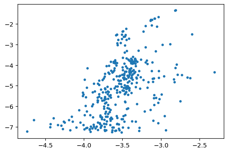
plt.plot(stellar_emulator.sigma_widths.detach().cpu(), stellar_emulator.amplitudes.detach().cpu(), '.')

[18]:

[<matplotlib.lines.Line2D at 0x7feb8d7a4610>]

../_images/paper_figures_WASP-69_HPF_paperfigs_27_1.png

Experiment to fine-tune line wings

[19]:

#with torch.no_grad():
#    mask = stellar_emulator.amplitudes > -2
#    stellar_emulator.gamma_widths[mask] = -1.
#    stellar_emulator.amplitudes[mask] = -0.5
#    stellar_emulator.sigma_widths[mask] = -1.5

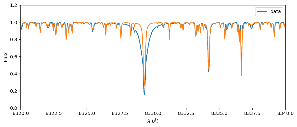
Initialization#

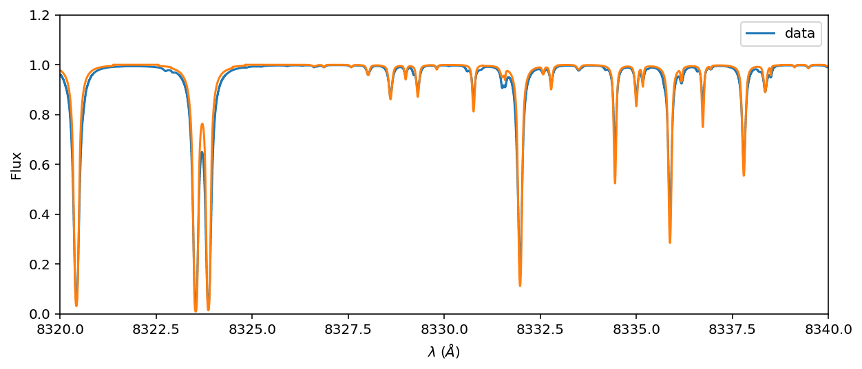
[20]:

ax = spectrum.plot(label='data')
ax.plot(stellar_emulator.wl_native.cpu(), stellar_emulator.forward().detach().cpu())
ax.set_xlim(8320, 8340);
ax.set_ylim(0, 1.2)
ax.legend(ncol=3);

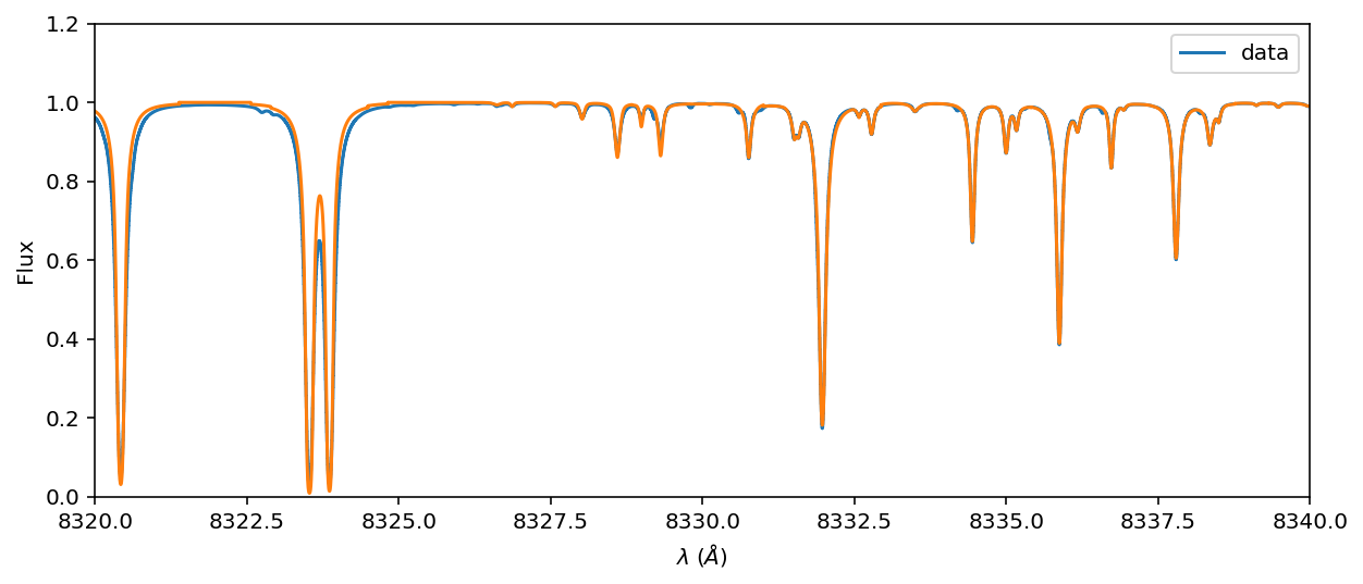
../_images/paper_figures_WASP-69_HPF_paperfigs_31_0.png

Fine-tune the clone#

[21]:

stellar_emulator.optimize(epochs=1000, LR=0.01)

Training Loss: 0.00012634: 100%|███████████| 1000/1000 [00:05<00:00, 191.29it/s]

[ ]:

[22]:

ax = spectrum.plot(label='data')
ax.plot(stellar_emulator.wl_native.cpu(), stellar_emulator.forward().detach().cpu())
ax.set_xlim(8320, 8340);
ax.set_ylim(0, 1.2)
ax.legend(ncol=3);

../_images/paper_figures_WASP-69_HPF_paperfigs_35_0.png

[ ]:

[23]:

ax = telluric_spectrum.plot(label='data')
ax.plot(telluric_emulator.wl_native.cpu(), telluric_emulator.forward().detach().cpu())
ax.set_xlim(8320, 8340);
ax.set_ylim(0, 1.2)
ax.legend(ncol=3);

../_images/paper_figures_WASP-69_HPF_paperfigs_37_0.png

[ ]:

[24]:

telluric_emulator.optimize(epochs=1000, LR=0.01)

Training Loss: 0.00001187: 100%|███████████| 1000/1000 [00:04<00:00, 217.21it/s]

[25]:

ax = telluric_spectrum.plot(label='data')
ax.plot(telluric_emulator.wl_native.cpu(), telluric_emulator.forward().detach().cpu())
ax.set_xlim(8320, 8340);
ax.set_ylim(0, 1.2)
ax.legend(ncol=3);

../_images/paper_figures_WASP-69_HPF_paperfigs_40_0.png

Step 3: Extrinsic model#

[26]:

extrinsic_layer = ExtrinsicModel(wavelength_grid, device=device)
vsini = torch.tensor(vsini)
extrinsic_layer.ln_vsini.data = torch.log(vsini)
extrinsic_layer.to(device)

[26]:

ExtrinsicModel()

(Remap the stellar and telluric emulator to a standardized wavelength grid).

[27]:

stellar_emulator = SparseLogEmulator(wavelength_grid,
                                     init_state_dict=stellar_emulator.state_dict(), device=device)

Initializing a sparse model with 361 spectral lines

[28]:

with torch.no_grad():
    stellar_flux_orig = stellar_emulator.forward()
    broadened_flux_orig = extrinsic_layer(stellar_flux_orig)
    telluric_attenuation_orig = telluric_emulator.forward()

[29]:

stellar_emulator.radial_velocity.data = torch.tensor(observed_RV)
stellar_emulator.to(device)
telluric_emulator = SparseLogEmulator(wavelength_grid,
                                     init_state_dict=telluric_emulator.state_dict(), device=device)
telluric_emulator.to(device)

Initializing a sparse model with 178 spectral lines

[29]:

SparseLogEmulator()

[30]:

with torch.no_grad():
    stellar_flux = stellar_emulator.forward()
    broadened_flux = extrinsic_layer(stellar_flux)
    telluric_attenuation = telluric_emulator.forward()

[ ]:

Joint telluric and stellar model#

[31]:

flux_at_telescope = broadened_flux * telluric_attenuation

Instrumental model#

[32]:

instrumental_model = InstrumentalModel(data.bin_edges.value, wavelength_grid, device=device)
instrumental_model.to(device)

[32]:

InstrumentalModel(
  (linear_model): Linear(in_features=15, out_features=1, bias=True)
)

[33]:

instrumental_model.ln_sigma_angs.data = torch.log(torch.tensor(0.064))

[34]:

with torch.no_grad():
    detector_flux_orig = instrumental_model.forward(flux_at_telescope)

[35]:

detector_flux = instrumental_model.forward(flux_at_telescope)

[36]:

ax = data.plot(yhi=1.1)
ax.step(data.wavelength, detector_flux.detach().cpu().numpy());
#ax.set_xlim(8320, 8340)

../_images/paper_figures_WASP-69_HPF_paperfigs_56_0.png

Transfer learn a semi-empirical model#

Here we compare the resampled joint model to the observed data to “transfer learn” underlying super resolution spectra.

[37]:

from torch import nn
from tqdm import trange
import torch.optim as optim

[38]:

data_target = torch.tensor(
    data.flux.value.astype(np.float64), device=device, dtype=torch.float64
)

data_wavelength = torch.tensor(
    data.wavelength.value.astype(np.float64), device=device, dtype=torch.float64
)

[39]:

loss_fn = nn.MSELoss(reduction="mean")

Fix certain parameters, allow others to vary#

As we have seen before, you can fix parameters by “turning off their gradients”. We will start by turning off ALL gradients. Then turn on some.

[40]:

stellar_emulator.amplitudes.requires_grad = True
stellar_emulator.radial_velocity.requires_grad = True
stellar_emulator.sigma_widths.requires_grad = False
stellar_emulator.gamma_widths.requires_grad = False
telluric_emulator.amplitudes.requires_grad = True
telluric_emulator.sigma_widths.requires_grad = False
telluric_emulator.gamma_widths.requires_grad = False
telluric_emulator.lam_centers.requires_grad = False
instrumental_model.ln_sigma_angs.requires_grad = True

[41]:

optimizer = optim.Adam(
    list(filter(lambda p: p.requires_grad, stellar_emulator.parameters()))
    + list(filter(lambda p: p.requires_grad, telluric_emulator.parameters()))
    + list(filter(lambda p: p.requires_grad, extrinsic_layer.parameters()))
    + list(filter(lambda p: p.requires_grad, instrumental_model.parameters())),
    0.01,
    amsgrad=True,
)

[42]:

n_epochs = 2000
losses = []

Regularization is fundamental#

The blase model as it stands is too flexible. It must have regularization to balance its propensity to overfit.

First, we need to assign uncertainty to the data in order to weigh the prior against new data:

[43]:

# We need uncertainty to be able to compute the posterior
# Assert fixed per-pixel uncertainty for now
per_pixel_uncertainty = torch.tensor(0.01, device=device, dtype=torch.float64)

Then we need the prior. For now, let’s just apply priors on the amplitudes (almost everything else is fixed). We need to set the regularization hyperparameter tuning.

[44]:

stellar_amp_regularization = 5.1
telluric_amp_regularization = 5.1

[45]:

import copy

[46]:

with torch.no_grad():
    stellar_init_amps = copy.deepcopy(stellar_emulator.amplitudes)
    telluric_init_amps = copy.deepcopy(telluric_emulator.amplitudes)

# Define the prior on the amplitude
def ln_prior(stellar_amps, telluric_amps,):
    """
    Prior for the amplitude vector
    """
    amp_diff1 = stellar_init_amps - stellar_amps
    ln_prior1 = 0.5 * torch.sum((amp_diff1 ** 2) / (stellar_amp_regularization ** 2))

    amp_diff2 = telluric_init_amps - telluric_amps
    ln_prior2 = 0.5 * torch.sum((amp_diff2 ** 2) / (telluric_amp_regularization ** 2))

    return ln_prior1 + ln_prior2

[47]:

t_iter = trange(n_epochs, desc="Training", leave=True)
for epoch in t_iter:
    stellar_emulator.train()
    telluric_emulator.train()
    extrinsic_layer.train()
    instrumental_model.train()

    stellar_flux = stellar_emulator.forward()
    broadened_flux = extrinsic_layer(stellar_flux)
    telluric_attenuation = telluric_emulator.forward()
    flux_at_telescope = broadened_flux * telluric_attenuation
    detector_flux = instrumental_model.forward(flux_at_telescope)

    loss = loss_fn(detector_flux / per_pixel_uncertainty, data_target / per_pixel_uncertainty)
    loss += ln_prior(stellar_emulator.amplitudes, telluric_emulator.amplitudes)
    loss.backward()
    optimizer.step()
    optimizer.zero_grad()
    t_iter.set_description("Training Loss: {:0.8f}".format(loss.item()))

Training Loss: 5.50831121: 100%|████████████| 2000/2000 [02:38<00:00, 12.65it/s]

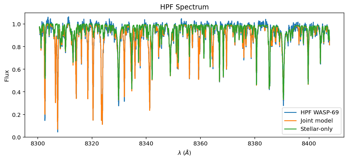
Spot check the transfer-learned joint model#

[48]:

ax = data.plot(yhi=1.1, label='HPF WASP-69')
ax.step(data.wavelength, detector_flux.detach().cpu().numpy(), label='Joint model');
ax.step(data.wavelength, instrumental_model.forward(broadened_flux).detach().cpu().numpy(),
       label='Stellar-only');
ax.legend()

[48]:

<matplotlib.legend.Legend at 0x7feb981aa370>

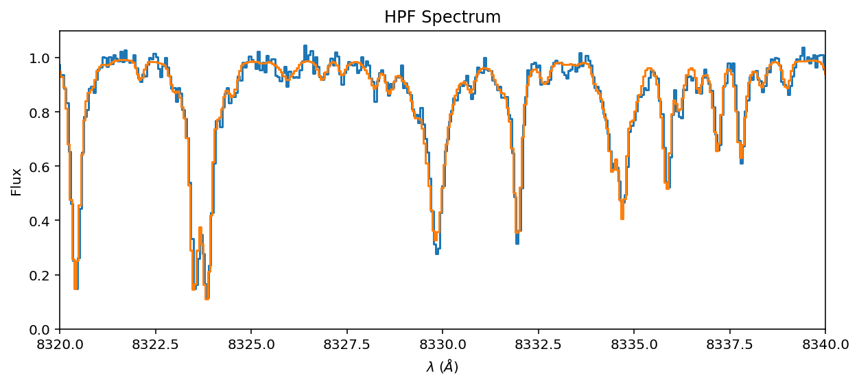
../_images/paper_figures_WASP-69_HPF_paperfigs_74_1.png

[49]:

ax = data.plot(yhi=1.1)
ax.step(data.wavelength, detector_flux.detach().cpu().numpy());
ax.set_xlim(8320, 8340)

[49]:

(8320.0, 8340.0)

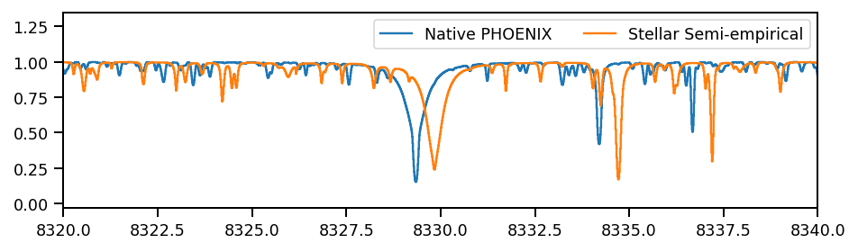
../_images/paper_figures_WASP-69_HPF_paperfigs_75_1.png

Inspect the individual stellar and telluric components#

[50]:

with torch.no_grad():
    #stellar_emulator.radial_velocity.data *=0
    stellar_post = stellar_emulator.forward().cpu().numpy()
    telluric_post = telluric_emulator.forward().cpu().numpy()

[51]:

import seaborn as sns

[52]:

sns.set_context('paper')

[53]:

fig, ax = plt.subplots(figsize=(7.5, 2))
spectrum.plot(ax=ax, ylo=0, yhi=1.1, label='Native PHOENIX')
ax.step(wavelength_grid, stellar_post, label='Stellar Semi-empirical');
#ax.step(wavelength_grid, telluric_post, label='Telluric Semi-empirical');
ax.legend(ncol=3)
ax.set_xlim(8320, 8340);
ax.set_ylim(-0.03, 1.35)
#ax.axhline(0, color='k', linestyle='solid', alpha=0.3)
plt.savefig('../../paper/paper1/figures/WASP_69_stellar_post.pdf', bbox_inches='tight')

../_images/paper_figures_WASP-69_HPF_paperfigs_80_0.png

Make a multi-panel plot#

We want 6 total panels, including one for initial data-model comparison#

[60]:

fig, axes = plt.subplots(nrows=6, figsize=(7.5, 7.5), sharex=True, squeeze=True)


ylo, yhi = 0, 1.15

ax = axes[0]
spectrum.plot(ax=ax, ylo=0, yhi=1.1, label='Native PHOENIX', color='#95a5a6')
ax.step(wavelength_grid, stellar_flux_orig.cpu(), label='blasé Clone', color='#c0392b')
ax.set_ylim(ylo, yhi)
ax.set_yticks([0, 0.5, 1])
ax.legend(loc=(0.22, 0.05))

ax = axes[1]
telluric_spectrum.plot(ax=ax, ylo=0, yhi=1.1, label='Native TelFit', color='#95a5a6')
ax.step(telluric_spectrum.wavelength.value, telluric_attenuation_orig.cpu(),
        label='blasé Clone', color='#2980b9')
ax.set_ylim(ylo, yhi)
ax.set_yticks([0, 0.5, 1])
ax.legend(loc=(0.22, 0.05))

ax = axes[2]
data.plot(ax=ax, ylo=0, yhi=1.1, label='HPF Data', color='#2c3e50')
ax.step(data.wavelength.value, detector_flux_orig.cpu().numpy(), label='blasé Model (initial)', color='#8e44ad')
ax.set_ylim(ylo, yhi)
ax.set_yticks([0, 0.5, 1])
ax.set_ylabel('Normalized Flux')
ax.legend(loc=(0.22, 0.05))

ax = axes[3]
data.plot(ax=ax, ylo=0, yhi=1.1, label='HPF Data', color='#2c3e50')
ax.step(data.wavelength.value, detector_flux.detach().cpu().numpy(), label='blasé Model (fit)', color='#8e44ad')
ax.set_ylim(ylo, yhi)
ax.set_yticks([0, 0.5, 1])
ax.legend(loc=(0.22, 0.05))

ax = axes[4]
spectrum.rv_shift(observed_RV).plot(ax=ax, ylo=0, yhi=1.1, label='Native PHOENIX', color='#95a5a6')
ax.step(wavelength_grid, stellar_post, label='blasé Semi-empirical', color='#c0392b');
#ax.step(wavelength_grid, telluric_post, label='Telluric Semi-empirical');
ax.legend(loc=(0.22, 0.05), title='[RV-shifted]')
ax.set_xlim(8320, 8340);
ax.set_ylim(ylo, yhi)

ax = axes[5]
telluric_spectrum.plot(ax=ax, ylo=0, yhi=1.1, label='Native TelFit', color='#95a5a6')
ax.step(wavelength_grid, telluric_post, label='blasé Semi-empirical',  color='#2980b9');
#ax.step(wavelength_grid, telluric_post, label='Telluric Semi-empirical');
ax.legend(loc=(0.22, 0.05))
ax.set_xlim(8320, 8340);
ax.set_ylim(ylo, yhi)
ax.set_xlabel('$\lambda ~ (\AA)$')

fig.subplots_adjust(0,0,1,1,0,0)
plt.savefig('../../paper/paper1/figures/WASP_69_multi.pdf', bbox_inches='tight')

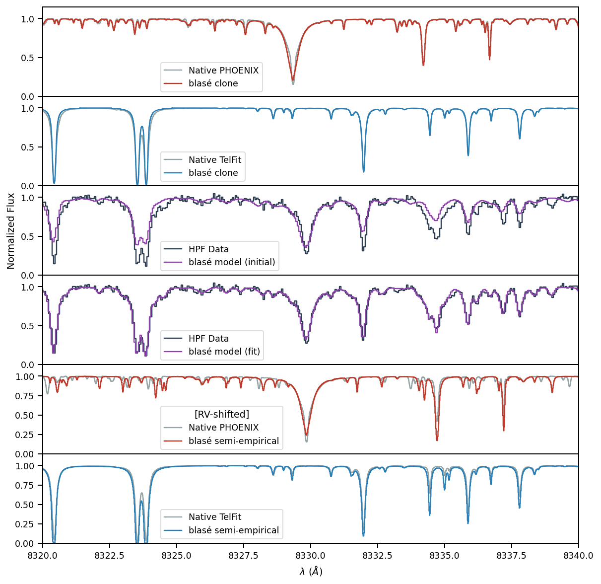
../_images/paper_figures_WASP-69_HPF_paperfigs_83_0.png

Nice!! This is the winner. Let’s keep it.

WASP-69 with HPF Paper Figures:

Contents