Step 4: Joint star and telluric model#
We now combine Steps 1, 2, and 3 to form a joint model for both the star and telluric atmosphere.
[1]:
import torch
from blase.emulator import (SparseLinearEmulator, SparseLogEmulator,
                            ExtrinsicModel, InstrumentalModel)
from blase.utils import doppler_grid
import matplotlib.pyplot as plt
import math
%config InlineBackend.figure_format='retina'
[2]:
wl_lo = 11_000-60
wl_hi = 11_180+60
wavelength_grid = doppler_grid(wl_lo, wl_hi)
[3]:
if torch.cuda.is_available():
    device = "cuda"
else:
    device = "cpu"
We will fetch the pretrained stellar model, following the previous tutorial.
Step 1: Clone the stellar spectrum
[4]:
stellar_pretrained_model = torch.load('phoenix_clone_T4700g4p5_prom0p01_11000Ang.pt')
stellar_emulator = SparseLinearEmulator(wavelength_grid,
                                        init_state_dict=stellar_pretrained_model)
stellar_emulator.to(device)
stellar_emulator.radial_velocity.data = torch.tensor(+25.1)
Initializing a sparse model with 426 spectral lines
Step 2: Clone the Earth’s atmosphere spectrum
[5]:
telluric_pretrained_model = torch.load('telfit_clone_temp290_hum040_prom0p01_11000Ang.pt')
telluric_emulator = SparseLogEmulator(wavelength_grid,
                                        init_state_dict=telluric_pretrained_model)
telluric_emulator.to(device)
Initializing a sparse model with 265 spectral lines
[5]:
SparseLogEmulator()
Step 3: Apply \(v\sin{i}\) broadening and RV shifting
[6]:
extrinsic_layer = ExtrinsicModel(wavelength_grid, device=device)
vsini = torch.tensor(1.1)
extrinsic_layer.ln_vsini.data = torch.log(vsini)
Compute the forward models at all three steps so far:
[7]:
stellar_flux = stellar_emulator.forward()
broadened_flux = extrinsic_layer(stellar_flux)
telluric_attenuation = telluric_emulator.forward()
The Earth’s atmosphere predictably attenuates the starlight#
Starlight impinges upon the Earth’s upper atmosphere as an extrinisically-modulated yet otherwise-pristine high resolution spectrum. The Earth’s atmosphere takes metaphorical bites out of this spectrum at high spectral resolution.
It is this composite stellar spectrum times telluric spectrum that arrives through the telescope dome and reflects into the instrument. We will refer to this flux as the “flux at the telescope” to distinguish it from the flux at the detector.
Step 4: Jointly model the star emergent spectrum and Earth’s attenuation.
[8]:
flux_at_telescope = broadened_flux * telluric_attenuation
[9]:
plt.figure(figsize=(8, 5))
plt.fill_between(wavelength_grid, broadened_flux.detach().cpu().numpy(), 1,
                 alpha=0.2, color='#f1c40f')
plt.plot(wavelength_grid, broadened_flux.detach().cpu().numpy(), color='#f39c12', lw=2, label='Star')
plt.fill_between(wavelength_grid, telluric_attenuation.detach().cpu().numpy(), 1,
                 label='Telluric Attenuation', color='#7f8c8d',alpha=0.2, step='mid')
plt.step(wavelength_grid, flux_at_telescope.detach().cpu().numpy(),
         label='Flux entering telescope',
         color='k', lw=2)

plt.xlabel('$\lambda (\AA)$', fontsize=12);plt.ylabel('Signal strength')
plt.xlim(11_020, 11_035); plt.ylim(0, 1.0)
plt.legend(loc='best', ncol=2);
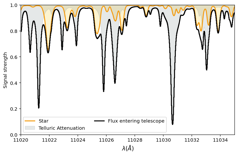
Excellent! The thick black line constitutes the joint model of stellar and telluric flux. In this view, most of the spectral structure arises from telluric lines, and the stellar lines are systematically blurred by their finite \(v\sin{i}\).
In the next tutorial, we will convolve the entire joint model with an instrumental kernel, and then resample it onto wavelength coordinates dictated by a data spectrum.