Step 5: Instrument broadening and resampling

We now apply the fifth and final step of the model creation process: applying instrumental modulation.

We will first apply steps 1, 2, 3, and 4 to form a joint model for both the star and telluric atmosphere. Then we apply an instrumental model layer.

import torch
from blase.emulator import (SparseLinearEmulator, SparseLogEmulator,
                            ExtrinsicModel, InstrumentalModel)
from blase.utils import doppler_grid
import matplotlib.pyplot as plt
import math
%config InlineBackend.figure_format='retina'

wl_lo = 11_000-60
wl_hi = 11_180+60
wavelength_grid = doppler_grid(wl_lo, wl_hi)

if torch.cuda.is_available():
    device = "cuda"
else:
    device = "cpu"

Apply Steps 1, 2, 3, and 4 to get the flux entering the telescope

We will copy the code verbatim from last time for clarity.

Step 1: Clone the stellar spectrum

stellar_pretrained_model = torch.load('phoenix_clone_T4700g4p5_prom0p01_11000Ang.pt')
stellar_emulator = SparseLinearEmulator(wavelength_grid,
                                        init_state_dict=stellar_pretrained_model)
stellar_emulator.radial_velocity.data = torch.tensor(+25.1)
stellar_emulator.to(device)

Initializing a sparse model with 426 spectral lines

SparseLinearEmulator()

Step 2: Clone the Earth’s atmosphere spectrum

telluric_pretrained_model = torch.load('telfit_clone_temp290_hum040_prom0p01_11000Ang.pt')
telluric_emulator = SparseLogEmulator(wavelength_grid,
                                        init_state_dict=telluric_pretrained_model)
telluric_emulator.to(device)

Initializing a sparse model with 265 spectral lines

SparseLogEmulator()

Step 3: Apply \(v\sin{i}\) broadening and RV shifting

extrinsic_layer = ExtrinsicModel(wavelength_grid, device=device)
vsini = torch.tensor(1.1)
extrinsic_layer.ln_vsini.data = torch.log(vsini)
extrinsic_layer.to(device)

ExtrinsicModel()

Forward model Steps 1$-$3.

stellar_flux = stellar_emulator.forward()
broadened_flux = extrinsic_layer(stellar_flux)
telluric_attenuation = telluric_emulator.forward()

Step 4: Jointly model the star emergent spectrum and Earth’s attenuation.

flux_at_telescope = broadened_flux * telluric_attenuation

We now move the fifth and final step…

Philosophical Aside: Instrumental effects

by gully

Every spectrograph is characterized by a finite resolving power, \(R\equiv \frac{\lambda}{\delta \lambda}\). In the pathological limit of inifite resolving power \(\lim_{R\to \infty}\) the spectrum recorded at the detector would identically resemble the flux coming into the telescope. This unvarnished spectrum would possess no trace that the spectrum had interacted with a measurement aparatus.

Instead, real instruments conduct Acts of Destruction. Here is a partial list:

1. Blur the spectrum in a characteristic and predictable way

2. Integrate and resample the spectrum onto discrete pixel coordinates.

3. Warp spectral shapes based on wavelength dependent losses and throughputs

4. Add detector noise

blasé currently models Acts 1, 2, and 3 in the InstrumentalModel class. The detector noise gets handled later in likelihood-based inference.

Instrumental Blurring

A common heuristic is that the character of the blurring process is roughly Gaussian, with a fixed FWHM \(\approx \frac{\bar\lambda}{\bar R}\) across a limited bandwidth. Such heuristics appear adequate for most purposes, and so we adopt them here. These assumptions are imprecise at the high signal-to-noise ratio and large bandwidths of modern spectrographs, though, and we here at blasé aspire one day to push the envelope on the extent to which subtle instrumental modulations could be built into this step.

Resampling

blasé does one slightly non-standard step in the resampling process. Rather than accept a list of pixel center coordinates, we demand that the user provide the list of pixel bin edges. For most applications, these can be arrived upon by simply assuming an average pixel width \(w\) and placing the pixel edges at \(\pm \frac{w}{2}\). But in other cases the bin edges are unevenly spaced, or there may be gaps between pixels. blasé specifically anticipates a future in which this information is more widely available. Luckily, specutils already provides an easy-to-use attribute bin_edges to input these non-standard coordinates.

Let’s fetch some HPF data to get a demo with real-world bin edges.

from muler.hpf import HPFSpectrum

path = 'https://github.com/OttoStruve/muler_example_data/raw/main/HPF/01_A0V_standards/'
filename = 'Goldilocks_20210801T083618_v1.0_0036.spectra.fits'
raw_spectrum = HPFSpectrum(file = path+filename, order=20)

data = raw_spectrum.remove_nans().trim_edges().sky_subtract()

Notice that the bin_edges have one more element than the wavelength centers. A data spectrum with \(N\) pixels will have \(N+1\) bin edges.

len(data.wavelength), len(data.bin_edges)

(2040, 2041)

Step 5: Apply the instrumental broadening and resampling.

instrumental_model = InstrumentalModel(data.bin_edges.value, wavelength_grid)
instrumental_model.to(device)

InstrumentalModel(
  (linear_model): Linear(in_features=15, out_features=1, bias=True)
)

instrumental_model.ln_sigma_angs.data = torch.log(torch.tensor(0.084))

detector_flux = instrumental_model.forward(flux_at_telescope)

We finally have a complete forward model in 5 steps, resulting in our tunable prediction for what a data spectrum should look like given all known physical properties.

plt.figure(figsize=(8, 5))
plt.step(wavelength_grid, flux_at_telescope.detach().cpu().numpy(),
         label='Flux at telescope', color='#c0392b')
plt.step(data.wavelength, detector_flux.detach().cpu().numpy(),
         label='Instrument smoothed and resampled', color='k', lw=2)

plt.xlabel('$\lambda (\AA)$', fontsize=12);plt.ylabel('Signal strength')
plt.xlim(11_025, 11_032); plt.ylim(0, 1.0)
plt.legend(loc='best', ncol=2);

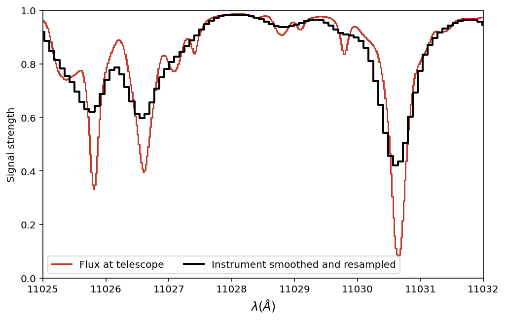
Phew! We have completed all five steps to create a forward model for astronomical spectra. You can see that the instrument-resampled model has much coarser sampling than the underlying input model.

Next stage: Data-model comparison…

The next stage is to compare this model to real data. The line properties can then be tuned en masse to fit the data spectrum– awesome!